Goal

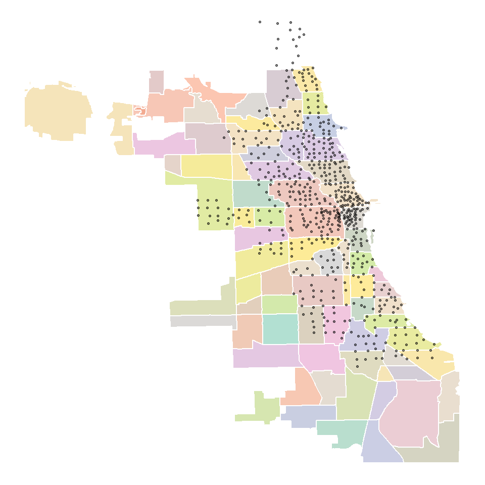
The goal of this post is to demonstrate how to overlay geographic points onto geographic polygons. Specifically, I’ll demonstrate how map the location of Chicago Divvy bike stations (points) onto the Chicago community map (polygons from a shapefile).

Data

Here is the data I used:

• The Chicago community boundaries came in a shapefile.
• The divvy station data contains the latitidue and longitude of all the Divvy bike stations in the Chicago area.

Example

library(rgdal)
library(readr)
library(broom)
library(RColorBrewer)
library(ggplot2)
library(dplyr)
theme_set(theme_void())

To read the shapefile, I use readOGR {rgdal}.

NOTE: I extracted the .dbf, .prj, and .shx files to the data directory.

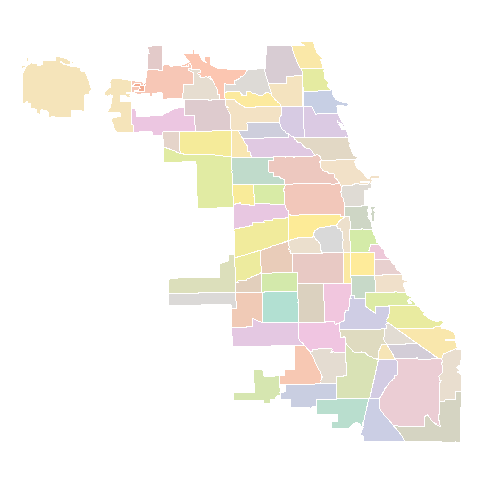
comm <- readOGR("./data/.")

Here is the code to create a plot of the Chicago communities:

# transform the shapefile data to a data.frame
comm.points <- tidy(comm)

# create a color palette, specifically a data.frame
# that maps a different color to each community id
colorCount = length(unique(comm.points$id))
getPalette = colorRampPalette(brewer.pal(9, "Set2"))
colors <- data.frame(
  id = unique(comm.points$id), 
  color = sample(getPalette(colorCount), colorCount))

# join colors to community ids
comm.points <- inner_join(comm.points, colors, by = "id")

# finally, plot the communities
ggplot(comm.points, aes(long, lat, group = group, fill = color)) + 
  geom_polygon(alpha = 0.5) +
  geom_path(color = "white") +
  coord_equal() +
  scale_fill_identity() +
  theme(axis.title = element_blank(), 
        legend.position = "none")

The tidy {broom} call simply extracts the polygon points into a data.frame. I had to add the special getPalette code because there were 77 different community ids and I wanted them to each have a separate color. So I created the colors data.frame to serve as a “lookup table” for each community’s color, which I used in the ggplot code.

Now, bring in the Divvy station data.

divvy <- read_csv("./data/Divvy_Bicycle_Stations.csv")

Now the tricky part. Plot the station locations on top of the community boundary map.

ggplot(comm.points, aes(long, lat, group = group, fill = color)) + 
  geom_polygon(alpha = 0.5) +
  geom_path(color = "white") +
  coord_equal() +
  scale_fill_identity() +
  theme(legend.position = "none") +
  geom_point(data=divvy, aes(Longitude, Latitude), inherit.aes = FALSE, alpha = 0.5, size = 0.5) + coord_equal()

It was important to tell geom_point not to inherit the aesthetics defined in the base layer. This is because geom_poly needed the fill and color aesthetics defined, but there was no grouping or color in the divvy data.

The coordinate_equal keeps the plot proportioned.

And, that’s it!